By Lawrence G. McMillan
This article was originally published in The Option Strategist Newsletter Volume 2, No. 23 on December 9, 1993.
We often speak of a position as being "statistically attractive". Many strategists who trade hedged positions have a vague idea of what that means, but would be hard pressed to cite specifics. In this issue, we're going to take a little more in-depth look at what, specifically, constitutes a statistical "edge". This will include looking at the way prices are distributed as well as delving further into the meaning and ramifications of volatility skewing. Then, we'll conclude by looking at a strategy that is currently popular in some circles.
In its broadest sense, the definition of "statistically attractive" merely means that a position has a positive expected return. That is, if one were to establish the same position over and over, he would expect to make a positive return (in excess of the risk-free rate). Obviously, in any one case or series of cases, the returns of the particular position or strategy could vary widely. Perhaps none of the actual returns in such a limited number of cases would be equal to the "expected return". Such practical limitations withstanding, this would not change the fact that the position has a positive expectation. Concentrating on positions with such positive expectations means one should be making a superior return over time.
One might ask, "Just what constitutes this positive expectation?" Since options lend themselves well to rigorous mathematical evaluation via a model, as option traders we often attempt to find positions in which we buy "undervalued" options and sell "overvalued" options against them. Such a strategy — if implemented properly — would be one way to produce a position with a positive expected return. Of course, we know in practice that it is not really all that easy to evaluate an option because of the difficulty in predicting the volatility of the underlying security.
A fairly "safe" way in which to identify options with different relative valuations is in the situations where volatility skewing exists. That is where different options on the same underlying security have different implied volatilities. A typical position would consist of buying options with lower implied volatility and selling options with higher implied volatility, both having the same instrument and their underlying security. The more common of these situations are broad-based U.S. Index options (where out-ofthe- money puts are more expensive than at- or in-the-money ones) and many of the grain and metals futures options (where the out-of-the-money calls are more expensive than other calls). The reason that volatility skew situations are especially attractive is that the projection of volatility of the underlying security — which is potentially the biggest source of evaluation error — is essentially irrelevant since any changes in future volatility would apply equally to both options in the position.
Distribution of Prices
The "backbone" of the expected return analysis and other statistical evaluations is the assumption that prices adhere to some distribution. That is, stock and futures prices (and other things, too, such as interest rates) move in a range that can be identified. One of the most common distributions is the normal distribution, or "Bell Curve". The graph below shows how a typical normal distribution looks; the fact that is shaped somewhat like a bell when viewed from the side explains the alternate name.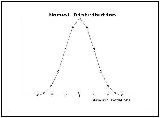
The interpretation of this graph is relatively straightforward: the height of the curve at any point is the probability of the stock moving that far. The stock initially starts at the point marked "0" on the chart. There is the greatest probability that it will be near that price after a specified length of time. However, there is some probability — albeit a much smaller one — that it could move 3 standard deviations up or down. In reality, of course, the stock or future can move more than three standard deviations, although the probabilities of its doing so are small.
The above graph has problems when it applies to financial prices, however, since it theoretically allows for stocks or futures to fall to negative prices. Thus, most analyses are done with a related distribution, the lognormal distribution, because it more directly applies to the way financial prices move. The graph at the top of the next column shows two lognormal distributions. Concentrate on the wider one, marked as "high volatility". The current stock is price 50; the point of highest probability occurs at 50. Notice that the lognormal graph is somewhat different from the "normal" graph on the left. The lognormal does not go below zero (therefore there cannot be negative stock prices), and it allows for stock prices to go significantly higher than their current price.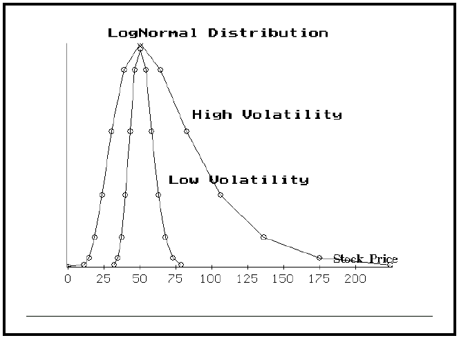
Volatility Important Here Also
Volatility is important in the distribution graphs also (it seems that we can never get away from estimating volatility, doesn't it?). The range of prices that a stock or future can trade within is, of course, related to the volatility of that stock or futures contract. Look again at the above graph. A second lognormal distribution lies within the wider one. This second one is much narrower, essentially implying that the stock prices would remain between about 30 and 80, while the "wider" curve indicates that stock prices under that distribution could range from as low as 10 to as high as 225!. What's the difference between these two curves? Volatility! The higher volatility stock obviously has a much greater potential trading range than does the lower volatility stock.
Volatility Skewing's True Meaning
Not everyone assumes that stock and futures prices are lognormally distributed (i.e., they adhere to a curve shaped like the ones in the above graph). However, whatever distribution one assumes, it is still the case that all options on the same underlying security should theoretically trade with essentially the same implied volatility. However, we all know that this is not the case when volatility skewing is present.
When volatility skewing is present, the options are describing a different distribution than actually exists in the marketplace. That is, the overpriced options are implying that there is a greater chance of something occurring than is actually the case; the underpriced options imply that there is less of a chance than there really is. A specific example using OEX options may help to illustrate this point.
Example: OEX is trading at 425. The following table shows the implied volatility of options at 4 various strikes (even when volatility skewing is present, the puts and calls at the same strike must have the same implied volatility; otherwise a riskless arbitrage opportunity presents itself). In addition, two other important columns of information are shown. The first, labeled "lognormal probability" is the actual probability of OEX being at the striking price at January expiration. The second, labeled "skewed probability" is the probability that is being implied by these current option prices.
Strike   Implied    Lognormal      Skewed
        Volatility  Probability  Probability
 400       17%          7%           17%
 415       15%         28%           31%
 425       13%         50%           50%
 440       11%         20%           16%
The lognormal probabilities are derived from the same formulae that were used to draw the lognormal curves on page 2. The "skewed probabilities" are distinctly different, however. The skew is implying that there is a much greater chance of OEX dropping to 400 or 415 than there really is. For instance, there is really a 7% chance that OEX will be below 400 at January expiration. However, the high level of implied volatility of the Jan 400 put is implying that there is a 17% chance of OEX dropping that far. There is a significant discrepancy between these two probabilities. Which one is right? If we are assuming lognormal distribution, then we have to assume that 7% is correct and 17% is not. Thus, we can conclude that it is statistically advantageous to sell the Jan 400 puts. Of course, we would have to hedge that sale in order to establish a neutral position. The skew in the above example also implies that there is a lesser chance of OEX rising to 440 than there actually is (20% versus 16%).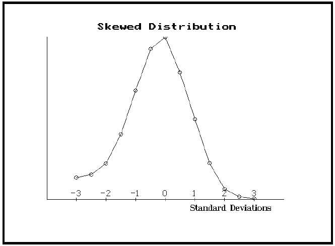
If the skew's probabilities were correct, a "normal curve" would look like the graph at the top of the next column. Notice that there is a raised "tail" on the left side of the curve now, and that the right hand side drops to zero more quickly. This is what volatility skewing is implying in the case of OEX options; but this distribution is not the true one that OEX prices follow. In order to take advantage of this distribution, one would buy options with higher strikes and sell options at lower strikes against them. This could be done with puts (resulting in ratio put spreads) or with calls (resulting in call backspreads).
The "Condor"
A strategy that is popular these days is the "condor" in which one sells an out-of-the-money combination on OEX — sell the Jan 440 call and the Jan 415 put for example — and hedges that sale by buying an even farther out-of-the-money combo (buy the Jan 445 call and the Jan 410 put to hedge). This results in two credit spreads, whose total credit probably would come to about 1¼ points before commissions. If OEX is between 415 and 440 at January expiration, one keeps the entire credit. The worst that can happen is that OEX rises above 445 or falls below 410 and the in-the-money spread has to be repurchased for a 5 point debit, plus commissions. The investment is 10 points of collateral, less the credit taken in from the initial sale.
This strategy is especially interesting in light of our discussion on expected returns and probabilities. The strategy is currently popular because it ostensibly has a phenomenal recent track record (which we have not verified). However, this strategy has a negative expected return after commissions are considered. Notice that with the current volatility skew in OEX options, the put portion of the "condor" is opposite to optimal strategy: one is buying the expensive put and selling the cheaper one. On the call side, the spread does align itself with optimal strategy, but the put spread is dominant because of the higher implied volatilities of the puts. Therefore, in the "condor" one is not selling anything more expensive than he is buying; in fact, he may be doing the opposite. When commission costs are added (and the possible costs of early assignment), the overall strategy has a negative expected return.
Has it been profitable? Yes. Will it continue to be profitable? Maybe, over the short term. Does it have a positive expectation? No. Therefore, somewhere in the future, this strategy can be expected to hit a long losing streak, probably when the actual price volatility of OEX increases, and the probability of OEX exceeding the maximum profit range of the spread becomes large.
Adherents of this strategy also make some adjustments, such as buying back the combination if OEX trades at the inside strike (close out if OEX hits 440 or 415 in the above example). This follow-up action virtually eliminates the chances of ever having to pay 5 points to buy back the spread, or of early assignment. However, it makes for a much larger probability of closing the spread at a loss in any one month.
These adherents are making money now, and of course are free to stop engaging in the strategy if the market should become volatile and start causing them losses. The point of the discussion is not to denigrate the "condor" strategy, but to point out that even strategies with negative expectations can have periods of time where they make money. The astute option strategist should realize, however, that one is best served to concentrate on strategies with positive expected returns. If he does this, he will not have to estimate market directions or future volatility changes in order to determine if he should continue to pursue his current strategy.
This article was originally published in The Option Strategist Newsletter Volume 2, No. 23 on December 9, 1993.

© 2023 The Option Strategist | McMillan Analysis Corporation