Selecting A Strategy (14:09)

By Lawrence G. McMillan

This article was originally published in The Option Strategist Newsletter Volume 14, No. 9 on May 12, 2005. 

Occasionally, options on a particular entity (usually a stock or, less frequently, an index) will become so skewed that they are actually skewed in two directions – both horizontally and vertically. We saw dually skewed situations with some frequency in the fall of 2002, when traders felt that there was substantial risk of near-term volatility (hence, a horizontal skew arose), coupled with the possibility of further large declines in stock prices (so a reverse, or negative, skew arose as well).

Since the market bottomed in late 2002 or early 2003 (take your pick), there have been very few reverse skews. Horizontal skews have remained somewhat prevalent – especially in the last year or so (witness the relatively large number of calendar spreads we have utilized in the “volatility trading” section since May, 2004). Many of those horizontal skews arise when a news event lies on the horizon – earnings, FDA hearing, etc.

However, there are still times when both skews are present simultaneously. In this article, we’re going to look at one such specific case and examine the various strategies that one might employ in this situation.

Network Appliance (NTAP) is due to report earnings on May 24th. That pending event has produced a horizontal skew in the NTAP options, with the June series having the highest implied volatility (since they are the contracts expiring closest after the “event” takes place). In addition, a reverse skew has developed – one in which the lower strikes have higher implied volatilities than the higher striking prices do. This is apparently because option traders fear a downside move could be substantial. Note that the stock itself has not been down a lot going into these earnings (chart, page 11). In other words, the option market is not predicting that the earnings will be bad, but is rather saying that a surprise on the downside would result in a much larger move than a positive earnings surprise would.

The actual data is listed in Table 1. The option prices listed are the average of bid and asked, while the implied volatilities are shown on the right. The put implied volatilities are not shown, but they adhere to a similar skew pattern. The stock itself was trading near 27-1/2 when these prices and implied volatilities were recorded.

First, notice the horizontal skew, by looking at any one strike – 25, say – and noticing the implied volatilities of the various months: Dec 48%, Sept 52%, and June 63%. This same pattern – highest implied volatilities in June, lowest in December (with September being between the two) – is what defines a horizontal skew. In general, since the “event” is taking place just before June expiration, the June options are much more expensive than the other two months. Hence a volatility trader would want to sell June options and buy either Sept or Dec options.

Second, there is a reverse (or negative) skew in these options as well. That means that the lowest strike has the highest volatility, and each higher strike has progressively lower volatilities. In the table, consider the June options. Reading from the lowest strike to the highest, the implied volatilities are 72%, 66%, 63%, 56%, and 51%. A similar pattern exists in the September and December options as well. Considering only this skew, one would want to buy options with higher strikes and sell options with lower strikes, if he were trying to establish a theoretically-based trade.

Since there is a dual skew in NTAP options, one can combine both skews in his strategy and would thus want to sell near-term June options with a low strike while buying longer-term options with a high strike. Such a trade would have the largest discrepancy in implied volatility between the options being used in the spread.

There are several strategies that follow this general guideline. For example a simple diagonal bearish spread would “fit:”
Buy 1 Dec 30 put at 5.00 (iv 46%)
and Sell 1 June 22.5 put at 0.50 (iv 66%)
While this spread certainly has an “edge” in implied volatilities, it is really little more than a long Dec 30 put, for the price of that put is so dominant in comparison to the fractionally-priced put being sold against it. For this reason, one might rather give away some of his “edge” in volatility in order to construct a spread with more neutral parameters. Perhaps something like the following would be a more reasonable approach:
Buy 1 Sept 25 put at 1.90 (iv 52%)
and Sell 1 June 22.5 put at 0.50 (iv 66%)
Now one has a position with a lower debit, a relatively large profit potential (percentagewise) and an edge in implied volatility.

Furthermore, it is likely that September options are more liquid than December options, which is another reason that a (large) trader might favor the September options over the December ones.

Even so, this example spread is quite bearish. It will certainly lose money if the stock rises in price. Rather one might prefer to establish a position in which a wider profit range, perhaps less directional in nature, can be established. While it is not necessary to be completely “delta neutral,” one often prefers less directional risk than the above simple spread entails.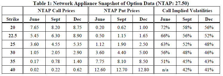

While there are many ways that more complicated spreads could be constructed, there are essentially three ways that are feasible: dual calendar spreads, a call backspread, or a put ratio spread. The latter two adhere strictly to what we want to do – buying long-term options with higher strikes, while selling shorter-term options with lower strikes. The dual calendar spread relies more heavily on the horizontal skew, but is still a feasible strategy.

All have their benefits, and so it will eventually fall to the strategist to select the one that best conforms with either his risk profile or what expectations he has for the stock’s movement after earnings are announced (if he has any at all).

Let’s discuss each briefly (the following analyses assume NTAP = 27.50 initially):

Diagonal Call Backspread

Buy 10 NTAP Sept 30 calls @ 2.10
Sell 5 NTAP June 22.5 calls @ 5.40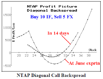

A call backspread typically has two features: 1) it is established for a credit, and 2) more options are owned than are sold. The “credit” feature means that the position will make money if the underlying falls dramatically, for all the options would expire worthless, leaving the spreader with a profit equal to the initial credit received. Furthermore, the presence of the excess long calls means that large profits would accrue if the underlying were to rally substantially. The profit graph of this particular spread is shown on the right, above. There are two profit curves on the graph: the first 14 days hence (just after the earnings are released) and the other at near-term, June expiration. Note that the position should make money in 14 days if the stock moves below 25.5 or above 31 – certainly possible given the past earnings reactions of NTAP. The margin for this spread is $3750 ($750 for each of 5 credit spreads) less the $600 credit of the spread, or $3150. We will discuss expected returns later.

Put Ratio Spread

Buy 10 NTAP Sept 25 puts @ 1.90
Sell 20 NTAP June 22.5 puts @ 0.50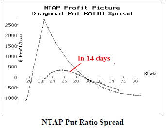

This put ratio spread is established for a debit of about $900. The profit graph is shown on the right (middle graph). Margin would be required for 10 naked puts, plus that initial debit. Clearly, this position has downside risk if the underlying should fall too far. However, since it does adhere to the skew criteria, it would probably be the best position if NTAP is relatively unchanged, or only slightly lower. However, if it were to fall below 20, large losses could occur.

Dual Calendar Spreads

Buy 10 Sept-June 30 Call Calendars @ 1.10
and Buy 13 Sept-June 22.5 Put Calendars @ 0.70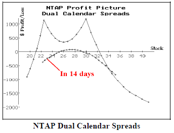

While a dual calendar spread does not really take advantage of the reverse skew – only the horizontal one – it still has a rather attractive picture. This position makes money if NTAP is between 21 and 32 at June expiration (see the above profit graph). The debit required for this position is approximately $2010 – all of which could be lost if the underlying makes a substantial move.

Expected Return

Now one must decide which of the three strategies to use. In theory, one could merely compare the expected returns of the three and choose the highest one. The annualized expected returns, at June expiration, of the above three spreads are:
Diagonal Call Spread: 9%
Put Ratio Spread: 124%
Dual Calendar Spread: 165%
Note: the expected return for the put ratio spread may vary with the movement of the underlying stock. Using these numbers, one would select the dual calendar spread. However, “expected return” assumes that the stock moves in a lognormal fashion. In this case, NTAP may move in an entirely different manner – it is likely to gap strongly one way or the other and then move lognormally after that.

Hence, one might decide to choose the strategy whose profit potential most closely fits with his expectations of movement in the underlying stock. This becomes more of a personal choice. Are you risk averse? Then perhaps the Diagonal Call Spread is best. Do you think the whole situation is over-hyped and the stock really won’t move much? Then the Dual Calendar Spreads may be best. We are going to recommend the Diagonal Call Spread:
Position E568: NTAP Diagonal Call Spread
Buy 10 NTAP Sept 30 calls (NULIF)
and Sell 5 NTAP June 22.5 calls (NULFX)
For a credit of 1.10 per 2-by-1 spread.
NTAP:28.67 Sept 30 call: 2.75 June 22 call: 6.50 The total margin required is $3750, less the credit received, plus commissions. We will look to remove the spread after the earnings are released, if possible.

This article was originally published in The Option Strategist Newsletter Volume 14, No. 9 on May 12, 2005.