
By Lawrence G. McMillan
This article was originally published in The Option Strategist Newsletter Volume 16, No. 7 on April 12, 2007.
This article reflects some new research (or, more appropriately, backtesting) that we have done regarding credit spread strategies. These strategies are very popular at the current time with a large number of web sites and advisory services. However, it seems that most people don’t really understand the risk that they’re taking in this strategy. Many stories are now surfacing about condor spread accounts with losses of 50%, 60% and more. Most of these were caused by being heavily invested in a month when the underlying made a maximum move.
For completeness, let’s start at the beginning. A credit spread involves buying one option and (simultaneously) selling another option – where the two options expire in the same month, but have different strikes. If the option that is sold is trading at a higher price than the option that is bought, a credit is taken in when the spread is established. Hence it is a credit spread.
Credit spreads can be either put spreads or call spreads. Generally, when these are initiated, they utilize out-of-the-money options. If one sells both an out-of-the-money put spread and an out-of-themoney call spread, it is called a Condor Spread.
The theory is that if one sells options that are far enough out of the money, they will likely expire worthless. The credit spread portion of the strategy comes into play because traders can define their risk by use of the credit spread. Hence one sells a deeply out-of-the-money option and then buys an even farther out-of-the-money option as protection, creating a credit spread. The credit spread strategy has a fair amount of leverage, too, depending on how far apart the strikes are, because it involves less margin than a naked option would.
In a previous issue – Volume 14, No. 7 – we wrote an article entitled “A Volatility-Based Approach to The Iron Condor Strategy.” The gist of the article was that, if one were to approach the condor spread strategy in an intelligent manner, he should routinely sell options that are a certain statistical distance out of the money each month. By “a statistical distance,” we mean that one uses the volatility of the underlying to select striking prices that are 1.0, 1.5 or 2.0 standard deviations out of the money. Those are the options that would be sold. Then the condor spread is completed by buying options that are 5, 10, or 20 points (or maybe even more) farther out of the money.
On the surface, this seems to be an excellent strategy – particularly if one uses options on a relatively non-volatile instrument such as the S&P 500 Index ($SPX). This is generally the preferred underlying for a vast majority of condor spreaders.
We backtested this strategy, testing a variety of standard deviations to set the short strikes and a variety of distances between the striking prices in the credit spreads. The results are summarized in Table 1. These results involve establishing one spread per month, from March 1993, through February 2007 – a total of 168 months. The condor was established every month on option expiration day, expiring in the next month.
         Table 1: Various Condor Approaches
Sdevs   Strike Diff   Gross Profit   Return
2          20          $ 3700          185%
2          10            2400          240%
2           5            1100          220%
1          20            5300          265%
1          10           –1800         –180%
1           5               0            0%
1          50           36000          720%
The far left column, “Sdevs” is the number of standard deviations that was used to calculate the short strike. This was done at each option expiration date, using $VIX as the volatility estimate over the one-month period until the next expiration date. “Strike Diff” is the difference in the strikes. “Gross Profit” is the total profit, before commissions, of the spreads over all 168 months. “Return” is the Gross Profit divided by the Strike Differential (times 100) – assuming that the Strike Differential is the investment required.
The option prices in Table 1 (credits) were estimated using the Black-Scholes model with a skew equal to the average skew at that time (puts are more expensive than calls, out of the money). It was also assumed that in every case, at least a minimal credit could be obtained: 0.15 for call spreads and 0.25 for put spreads, even if the theoretical, skewed prices did not agree. Finally, a commission of $1.25 per contract was applied. Fourteen years ago, rates were much higher than that; today they are slightly lower, but that seems like a fair average. Note: in attempting to estimate prices, it became evident just how important good execution is in this strategy. A few nickels here and there can add up to quite a bit of profit over time.
These results were arrived at by having no followup strategy. That is, the options were held all the way to expiration. In some cases, that meant that the maximum loss was taken. In fact, in every line of Table 1, the maximum loss was incurred at least once over the 14-year period (see Table 2).
One very obvious thing is evident from the table. The profit is larger the farther apart that the strikes are. Extrapolating this, one would conclude that naked option selling is probably a better strategy – that the expense of the long options in the condor spread is just a waste of money. Mitigating that is the peace of mind that the spread provides, as opposed to a naked option. Also, the margin requirement is lower for the condor spread, so the returns might be larger in the spread strategy, as opposed to naked option writing.
On the surface, these returns – except for the last line – are not large, considering they took 14 years to accumulate. Moreover, one could not sink all of his money into this strategy, for the risk each month is 100% of the investment. In other words, your brokerage firm only requires that you advance enough margin to cover the risk. So, if one were to have invested his entire account in the strategy, and if a volatile move were to occur, causing one to have to buy back either the put spread or the call spread at the maximum spread differential, the account would be wiped out.
Thus, one needs to be aware of the “Probability of Ruin.” Table 2 shows how often the maximum loss was taken in each strategy over the 14-year period.
        Table 2: Probability of Ruin
Sdevs  Strike Diff  Gross Pft   # Max Loss
2           20       $ 3700          1
2           10         2400          1
2            5         1100          1
1           20         5300          9
1           10        –1800         15
1            5            0         20
1           50        36000          6
Later, we will discuss money management, but for now, suppose that you had started out with the minimum requirement ($2000 for the 20-point Strike Differential, or $1000 for the 10-point, etc.). And further suppose that you just keep investing that amount each month, taking any excess profits out. Eventually, when the maximum loss occurs, you would have to come up with another $2000, say, to keep the strategy going. In fact, you’d have to do that as many times as the maximum loss occurred (right-hand column above). So the returns would be altered. Simplistically, your “investment” would be the “Strike Diff” (times 100) times (1 + “# Max Loss”).
Using this adjusted definition of “investment,” which is certainly not the optimum investment, but is at least a realistic approach, the Returns would then be:
            Table 3: Adjusted Returns
Sdevs   Strike   Gross Pft   # Max  Invest   Return
        Diff                  Loss
2       20       $ 3700       1     $4,000     108%
2       10         2400       1     $2,000      83%
2        5         1100       1     $1,000     110%
1       20         5300       9    $20,000      27%
1       10        –1800       15   $16,000      n/a
1        5            0       20   $10,500       0%
1       50        36000       6    $35,000      97%
Under these assumptions, the returns (Gross Profit divided by Investment) are more uniform – and not very good, considering that these are the total returns over a 14-year period.
Two Standard Deviations vs. One?
Using a two-standard deviation approach, the maximum loss would have occurred only once – September, 2001, when the World Trade Centers were attacked. 166 of the 168 months generated the maximum profit (there was a small loss in June, 2002, in the depths of that bear market). These represent the numbers you sometimes see in “hype” ads: 99% percent of trades profitable. Of course, one of the ones that wasn’t profitable, wiped out nearly 50 months of accumulated profits. Furthermore, at two standard deviations, there were many months where the credit generated was trivial – where the 40-cent minimum credit was used in the study. Thus, the dollars of Gross Profit are rather small compared to the one-standard deviation studies using wide strike differentials.
From a practical standpoint, two standard deviations is not a very workable strategy. As a result, most systematic practitioners of this strategy use 1 or 1.5 standard deviations to estimate the short strike.
Money Management
Figure 1 shows the cumulative profit graph for one of the strategies: one standard deviation, with 50 points between the strikes. The near-maximum loss months are shown in bold red. Note that once (June-July, 2002) there were back-toback months with the maximum loss. This will be important when we discuss money management.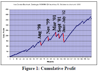
There were other times when losses were taken in the month, but not the maximum loss. Even then, though, one would have to add more money to his “investment” to continue the strategy, so the Adjusted Returns shown in Table 3 would, in practice, be even lower than estimated.
Even so, most observers would note that the maximum loss never occurred three months in a row, so they might try to devise a system of investment which allows for that fact to be coupled with the ability to reinvest some of the accumulated profits to date. This would allow one to be able to increase his investments substantially during a long winning streak. But would it produce better overall returns?
The following example shows one form of a generally accepted approach to money management; it may not be perfect Optimal f or exactly fit the Kelly Criterion1, but it is a reasonable facsimile.
   Example: Suppose you are considering implementing
   the condor strategy with a $50,000 account. Using
   strikes that are 20 points apart, you begin the strategy
   by allocating a third of your account ($16,667) to this
   strategy. The quantity of spreads that can be
   established would then be $16,667 divided by the
   margin required (risk).
   In reality, your investment is slightly smaller than
   $2,000 per spread; it is $2,000 less the net credit
   received when the condor spread is sold. Assume that
   the condor generates about $250 in credits per spread,
   so your net investment per spread would be $1,750.
   Thus you could establish about 9 spreads ($16,667
   divided by $1,750).
If you are into a winning streak, your account would be growing, and you would continue to risk one-third of your account each month. If a loss occurs, you cut back – still investing one third of what’s left after the loss.
Under this money management scenario, profits accumulate more rapidly, but losses are much nastier when they occur. One maximum loss costs you 33% of your account. If a second one occurs immediately in the next month, that’s a loss of 33% of the 67% of your account that remained, or another 22% of the original account. Hence, the back-to-back maximum losing months cost you 55% of your account. Even so, if you can build up a string of profits before that occurs – and if you can stomach those kinds of losses without abandoning your system – this is a way to accelerate the profits from this (or any other strategy).
Using this approach with the same strategy – one standard deviation to the short strike, and a 50-point striking price differential (the same criteria as in Figure 1), the cumulative profit graph now looks like this: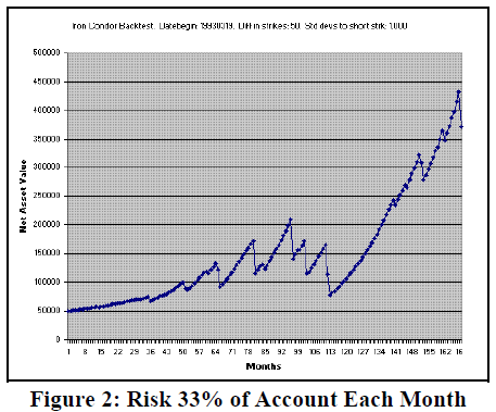
A $50,000 account has grown to over $372,000 (and was at $432,000 just before the March 2007 mini-crash in $SPX). Yet the initial risk in the first month was just $16,667 (33% of the initial asset value).
I am not claiming that 33% is the optimal risk, but this approach might just change the condor spread strategy from “trouble” to “worth the trouble.” At least with this approach, losses can be recouped in a shorter time.
We have also not addressed refinements of the followup strategy, such as closing the spread for the month if the underlying touches a striking price at which you have short options. When the strike differential is large, as in the above graph, that should be helpful as well. We will continue to research this concept in future articles.
In summary, the condor spread strategy can be a dangerous one, as many traders are now learning, but with proper money management, it can perform well.
This article was originally published in The Option Strategist Newsletter Volume 16, No. 7 on April 12, 2007.

© 2023 The Option Strategist | McMillan Analysis Corporation