
By Lawrence G. McMillan
This article was originally published in The Option Strategist Newsletter Volume 17, No. 17 on September 12, 2008.
We often get questions regarding the operation of volatility trading strategies. While we endeavor to explain why we are establishing certain trades, or why we are taking follow-up action, we really haven’t put it together in a sort of “how to” article. That’s the purpose of this week’s feature.
Many traders have no problem with figuring out what we’re doing with speculative positions and how we’re adjusting them (usually via a trailing stop, taking partial profits along the way and rolling up if the underlying gets too far ahead of its trailing stop). But the operation of a volatility trading strategy can be more difficult. For the purposes of the examples to be used in this article, we’ll discuss a dual calendar spread strategy. It’s been a successful strategy in this bear market, with these results in the last year – roughly since the onset of the bear market:
20 positions
12 winners (60%)
8 losers
Total gain, including commission: +$6,446
Average win: $829
Average loss: -$437
Average trade: +$322
Average investment: $2,383
Average holding period: 42 days
Average return, annualized: +118%
We generally use dual calendars when options are heavily skewed prior to an event taking place (normally earnings, although they could be used for FDA hearings, lawsuits, and other events). The reason that a dual calendar spread makes sense in such situations is that its profitability fits very well in the context of the expected stock price distribution of an “event-driven” trade.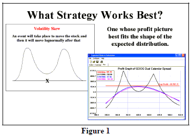
Figure 1 is a copy of one of the Powerpoint slides that we use in our seminar presentations on this subject. The curved line in the upper left of Figure 1 is the theoretical stock price distribution of an event trade: the stock starts at point “x.” Then an event causes the stock to either gap higher or lower, after which it moves in a lognormal fashion. So the distribution, from today’s viewpoint, actually looks like two lognormal distributions – one centered on the higher gap price and the other centered on the lower gap price.
A dual calendar spread utilizes a call calendar spread with a striking price higher than the current stock price, and also uses a put calendar spread with a striking price lower than the current stock price. It has a profit graph similar to the one shown in the lower right of Figure 1. The peaks of the dual calendar spread’s profitability are at the striking prices used – the higher one for the calls, and the lower one for the puts.
Notice how the two pictures inside Figure 1 are quite similar to each other. Thus, a dual calendar spread often fits the theoretical stock price distribution of an event-driven trade very well.
A dual calendar spread can be analyzed, in advance, using an Expected Return Calculator. There are two things we look for in a dual calendar spread, though, before even inputting the data into the calculator: 1) that there is a significant skew in the options (i.e, the near-term options are trading with implied volatilities at least 10% higher than the implied volatilities of the longer-term options), and 2) that the implied volatility of the longerterm options is not significantly higher than the “average” volatility of options in normal times.
A recent position that we established in Whirpool (WHR) options will serve as an example of the type of analysis that we use for such positions. We first noticed that WHR was appearing on our “skew list” in mid-July. This list appears daily on The Strategy Zone. It is constructed by calculating the standard deviation of the individual implied volatilities on the options of each stock, futures, or index. In a “normal” situation, the options on a particular stock will have very similar implied volatilities, and thus the standard deviation of the implieds would be very low. However, in a situation where the options are skewed, the standard deviation of implieds will be high. That is how the list is sorted – from high to low.
Once WHR was noted to be on the list, we then display a quote montage – using whatever quote system you have for option quotes – and note the implied volatilities of the WHR options. We use Realtick Turbo Options because the layout is conducive to spotting skews1. It was readily apparent that WHR August options were expensive with respect to longer-term WHR options. In general, the August calls had implieds in the high 50's, while December option implieds were in the mid-40's. We generally like to have two to four month’s time between the two months in our calendar spreads, so August vs. December is acceptable. This satisfies criterion (1) mentioned earlier.
In order to satisfy criterion (2), we need to have a chart of the implied volatility of WHR options, or at least have a table of percentiles so that we can decide if paying in the mid-40's for December options is a reasonable thing to do. Figure 2 (on page 3) is a chart of the implied volatility of WHR options, from the viewpoint of mid- July.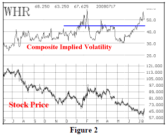
In Figure 2, the chart of daily composite implied volatility calculations is shown on top, and the daily stock price chart is shown below. The blue line is drawn at approximately the level of December option implied volatility (the mid-40's).
The options on WHR were expensive at the time because 1) earnings were due to be reported in about a week, and 2) the stock had been in decline for the previous five months. We need to decide if it’s reasonable to expect that December implieds will remain near or above the blue line after the earnings report has been issued. It’s not completely clear that they will. As you can see from Figure 2, the composite implieds had fallen as far as 30 in May, after the previous earnings report in April. On the other hand, with the stock in a general decline, it seems reasonable to assume that implieds would not return to their lows – at least not right away. So, this might not completely satisfy criterion (2), but it doesn’t violate it, either.
So, we proceed with an expected return analysis. With the stock at roughly 67, we will use a call calendar spread with a 75 strike, and a put calendar spread with a 60 strike. We select these strikes somewhat subjectively, but they are based on two things: 1) the near-term (August, in this case) options must be selling for at least 1.00, and 2) those strikes should encompass the near-term trading range of the stock. You can see from figure 2, that – since gapping down in April – WHR has not traded above 75 nor below 60.
This is the position being considered:
Buy 3 WHR Dec 75 calls: 5.00
Sell 3 WHR Aug 75 calls: 1.55
Buy 4 WHR Dec 60 puts: 4.90
Sell 4 WHR Aug 60 puts: 1.55
Total Debit: $2375
Usually, a ratio of about 3 call spreads to 4 put spreads is neutral. The easiest way to adjust this is to try to even out the two peaks in the profit graph that is generated by the Expected Return Calculator. Figure 3 shows that output. You can see that the peaks are about level at that ratio. If the call peak was higher, then you might try a ratio of 3 call spreads to 5 put spreads.
From Figure 3, you can see that the expected profit is $443 – a very desirable profit on an investment of $2375 for one month.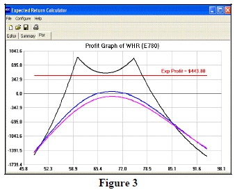
However, this is the point at which one needs to be very critical. That $443 expectation assumes that the December options will retain their current levels of implied volatility. But what if they don’t? How far can Dec vol fall before the expected profit disappears completely? This is an easy question to answer when you have an Expected Return Calculator at your disposal.
Just keep lowering the projected implied vols of the December options until the expected profit falls to zero. That is your “breakeven volatility” for the position. In this case, the “breakeven volatility” is about 41%. Looking once again at Figure 2, you can see that composite implied volatility has been above 41% for a considerable amount of time this year. So, we felt the position was worth establishing – as Position E780.
WHR reported earnings the next week, and they were positive. The stock gapped up to 77 on that news, but then stagnated in the 73-77 area for the rest of July. By the end of July, the position was marking at a small profit, and the stock was edging up towards 77 once again. If the stock were to break out to the upside, it would harm the profitability as the stock moved away from the 75 strike. Moreover, the composite implied volatility was down to 40%, so any move lower in December vol would hurt the position, too.
So, we gave instructions to close out the spread and take the profit. The position was closed on August 1st. It was a fortuitous decision, since the stock broke out over 75 a couple of days later and ran all the way to 84 by August expiration – when the spread would have had to been removed at a loss. By that time, composite implied volatility had fallen to 38%.
Our “official” records show a gain of only $59 after commissions, although it was possible to exit at a slightly better price than that. In any case, that is a high annualized return (the position was held for only two weeks). More importantly, though, this article has hopefully shown volatility traders how we analyze, scrutinize, trade, and close a dual calendar spread.
This article was originally published in The Option Strategist Newsletter Volume 17, No. 17 on September 12, 2008.

© 2023 The Option Strategist | McMillan Analysis Corporation