The Annual Intermarket Spread (19:19)

By Lawrence G. McMillan

This article was originally published in The Option Strategist Newsletter Volume 19, No. 19 on October 14, 2010.

Each year about this time, we review and recommend a futures spread that has been quite profitable over the years: buying Feb Gasoline futures and selling Feb Heating Oil futures. We call this an intermarket spread since it involves a long position in one market and a short position in a different, but related, market.

This spread has generally been quite reliable in the past, but it can only be implemented in one form – with the actual futures contracts themselves (more about that1 later). We have traded this spread almost every year since 1994, although the entry and exit parameters have been altered a few times.

In this article, we’ll take a detailed look at the track record of this spread and make a recommendation for implementing the spread this year. Figure 1 shows the historical relationship of the Feb Heating Oil contract minus the Feb Gasoline1 over a specific time period each year: from September 1st of one year through January 31st of the next year. Both contracts typically expire at the end of January.

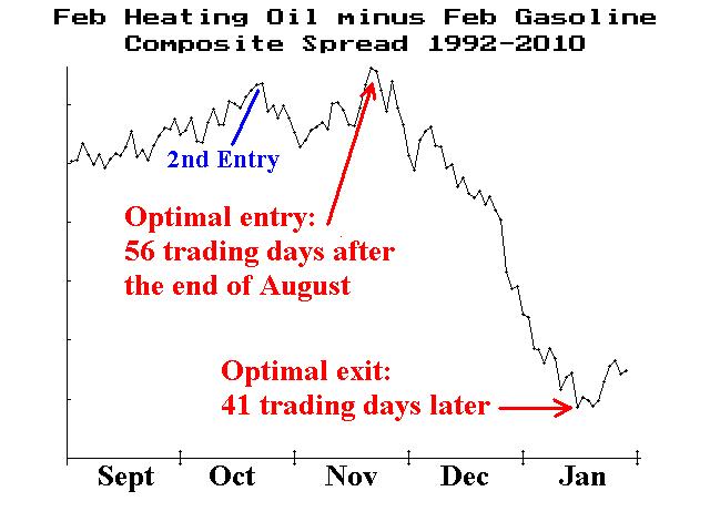
The data in Figure 1 encompasses contracts expiring in 1992 through those expiring in 2010 – nineteen years in total. There is no scale on the left side of the graph, because these contracts have traded at a wide variety of prices – and therefore the spread between the two has fluctuated over the years as well. Besides, it is the shape of the graph that is important.

From that shape you can see that Heating Oil slightly outperforms Gasoline until late November (the graph is slightly rising until then). After that, though, the graph plunges dramatically as Gasoline outperforms Heating Oil. It is this plunge that we want to capture, which means we will be buying Gasoline and selling Heating Oil, establishing the spread in late November and looking to exit in mid-January.

Specifically, the highest point on the graph in Figure 1 is 56 trading days after the end of August, and the low point is 41 trading days after that. Now, each year present a slightly different variation on the basic theme, but Figure 1 represents the average price of the spread on each trading day.

There are ETF’s for both of these products – heating oil (UHN) and gasoline (UGA) – but there are no options on UHN, so it wouldn’t make sense to implement the spread with a “pairs” trade in these ETFs, for the futures are more liquid. It is even theoretically possible to trade options on these futures instead of the futures themselves, but they are relatively illiquid and trade with such large premiums as to be unusable for our purposes.

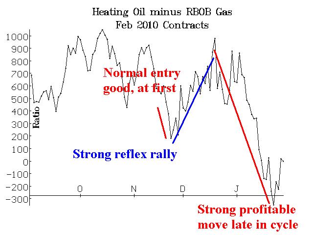
The smaller figures on the right and on page 3 show the spread as it performed in specific years – from this year (the 2010 graphs, since the futures expired in 2010), back through 2004. You can see that in each of these years, there was a significant profit available during December. However, even though we made money in most of those years, it was difficult to capture the full amount of the spread’s decline, since the optimal entry point shifted quite dramatically from one year to the next.

As a case in point, take last year (the 2010 graph). The best entry point was actually in early November, but we entered at the “optimal” time in late November – where the first red downward-sloping line begins. Shortly thereafter, the spread widened, creating unrealized losses (the rising blue line). Eventually, though, beginning in late December, the spread plunged, and we registered a profit on the trade.

Frankly, it was fortunate that we weren’t stopped out. In reality, there should probably be some contingency to exit a losing spread (limiting losses) but reenter if the spread turns around. The spread is volatile in that, even during trends, it can fluctuate quite wildly around the trend line. Therefore, using a trailing stop that is too tight could be counter-productive.

On the next page are graphs of the other recent years. In several of the graphs, the “alternate entry point” is referred to. That is shown in Figure 1, as a point in mid-to-late October. At one time in the past, that had been the optimal entry point, but it has moved to its current location in recent years. Even so, we have sometimes attempted to use both entry points. That has not worked well in several cases (see the chart on page 3), and therefore we are not going to use the secondary entry point any longer.

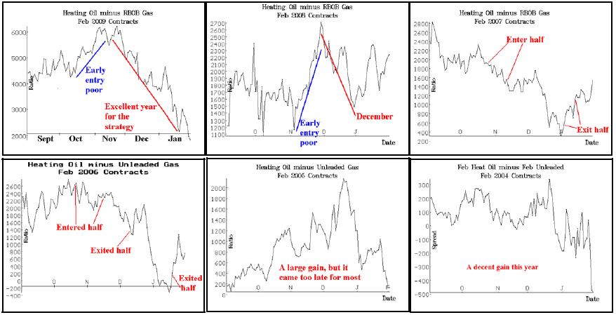
For a moment, ignore all data in the above charts, except for the month of December. You can see that, in every chart, the graph drops sharply at some point in December. In most of these years, we were able to profitably capture some of this decline, although in others it would have been almost impossible to do so.

Consider 2005, the middle chart in the lower row. The spread first exploded higher in early December – actually rising to new highs for that year – before eventually turning and falling sharply.

Something similar occurred in 2004, where the spread first expanded in the early part of December, and then collapsed in the latter half. In that year, we had entered the spread in October (the “old” optimal entry point), so we were able to withstand the December adverse move.

In the last five years, however, an entry point in late November has led to steady spread profits in December. Yes, there is still that slight adverse movement in the spread in early December, but it has been small in recent years.

The fact that this trade works most years seems to defy logic. After all, we are trading Gasoline from the long side, but that’s a product that see its greatest demand in the summer months, when families drive on weekends and on vacations. Heating Oil, on the other hand, is the product that we are short in this spread. Yet Heating Oil is greatly in demand in the winter, as many homeowners in the north use heating oil as a fuel for their furnaces. Hence it would seem that we are in exactly the wrong position. But history shows that we are not. The futures market apparently have already discounted the obvious by early December, and the spread begins to swing back the other way.

The simplest way to implement this spread is to buy the Gasoline futures and sell the Heating Oil futures. At most brokerage firms, this is considered a spread of sort and receive a bit of a favorable margin treatment. Each of these futures is worth $420 on a one point move, so each point of movement in the spread is worth $420.

In most intermarket spread situations, we use options, because that gives us two ways to make money: 1) on the convergence of the spread, or 2) if both underlyings make a volatile move in one direction or the other. In these products, however, the implied volatility is fairly high, so we would have to go so deeply in-themoney to eliminate time value premium expense, that it just isn’t worth it. These prices, which are near current prices, illustrate the problem: Feb HO: 235 Feb HO 250 put: 23.60 Feb RB: 217 Feb RB 200 call: 24.70 That is an onerous time value of 8.60 (put) + 7.70 (call).Currently, the spread is approximately 19.00, Heating Oil over RBOB. We want the spread to go negative (i.e., to have RBG1 trading at prices higher than HOG1).

This article was originally published in The Option Strategist Newsletter Volume 19, No. 19 on October 14, 2010.